
Calculus Without Tears
General Relativity
Introduction
The next time you are at a basketball game, and a player launches a long shot from the
 backcourt, you might muse aloud "Ah, Einstein was correct, spacetime IS curved." If the fan next to you questions your judgement (or sanity), you can reply ... "See the arc of the ball, it is following the curvature of spacetime, just as described in Einstein's general theory of relativity", and, you would be exactly right. The photo shows Kareem Abdul Jabbar preparing to demonstrate Einstein's general theory. We'll calculate the radius of curvature of Kareem's sky hook in spacetime below, and the answer may surprise you.
Minkowski Spacetime, The Equations of Weingarten, Christoffel Symbols of the First and Second Kind, the Ricci Tensor, the Theorema Egregium, the Riemann Curvature Tensor, and more! Where special relativity didn't require any calculus, general relativity is a smorgasbord of differential equations.
General relativity is primarily a theory of why things fall, it replaces Newton's theory of gravity. According to the general theory as proposed by Einstein, the apple falls from the tree not because of some mysterious invisible force called gravity, but because the spacetime around the apple is curved by the large mass of the earth. How can we 'visualize' the new theory? ... actually, we don't have to visualize it as we can actually see it with our own two eyes. Remember, when Kareem releases his sky hook, there is no gravity pulling it down. So, why does it fall? Because spacetime is curved, and the ball is actually following a geodesic, or straight line, in curved spacetime. The arc of the ball's trajectory is due to the curvature of spacetime ..... there it is.
Riemannian Geometry
The mathematics of general relativity is the mathematics of non-Euclidean curved space, and, remarkably, the mathematics was invented before the advent of relativity, the mathematics of curved space was initiated by Gauss and further developed by his student, Riemann. Gauss was studying the problem of drawing a flat map of the earth, he discovered that a perfect distance preserving flat map couldn't be drawn because the earth is a curved surface. Note that a distance preserving flat map of a cylindrical surface can be drawn by unrolling the cylinder, thus, a cylinder is not a curved surface! Riemann added to the theory of curved surfaces and this branch of mathematics is called Riemannian geometry; there is no avoiding it if we are going to understand general relativity.
If what follows seems a little complex, be consoled to know that it is only 'elementary' Riemannian geometry. And, really, it's mostly just differentiating local basis vectors, expressing the result in the local frame, and giving names to the vector components. I.e., it mostly straightforward differentiation, combined with rearranging the terms and naming new functions. Much of the apparent compexity comes from the sheer number of functions, even for a two-dimensional curved surface this proliferation can be daunting. Note that every one-dimensional curve has a straight line distance preserving map, and so we can't simplify matters further by reducing the dimension to one as there are no one-dimensional curved spaces.
Curves in Euclidean 3-Space
A curve in E3 is given by a vector valued function
a(t) = (x(t), y(t), z(t))
the velocity of the curve is
a'(t) = (x'(t), y'(t), z'(t))
and the acceleration is
a''(t) = (x''(t), y''(t), z''(t))
A curve can be reparameterized with the parameter s which is the arc length of the curve, so that
length(a'(s)) = 1. When a curve is parameterized with its arc length, then the acceleration of the curve measures how fast the direction of the velocity of the curve is changing, and the curvature of the curve is defined to be length(a''(s))
Example:
the curve a(s) = (R*sin(s/R), R*cos(s/R), 0) is a circle in the x-y plane with radius R. It is parameterized by arc length.
a'(s) = ((1/R)R*cos(s/R), -(1/R)R*sin(s/R), 0) and length(a'(s)) = 1, and,
a''(s) = (-(1/R)2R*sin(s/R), -(1/R)2R*cos(s/R), 0) and length(a''(s)) = 1/R
Thus, the curvature of a circle of radius R is 1/R. Seems right.
Curves in Surfaces in Euclidean 3-Space, 1st Derivative
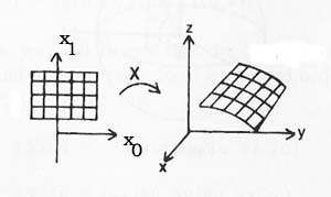 We will define a 2-d surface in E3 as the image of a vector valued function from a region in E2 to E3, eg,,
X(x0,x1) = (x(x0,x1), y(x0,x1), z(x0,x1))
With this definition, we get not only the surface itself, but also 2-d coordinates on the surface, with the coordinates of a point (a, b, c) on the surface equalling (x0,x1) where (a, b, c) = X(x0,x1)
A curve in the surface, parameterized by its arc length, is given by
a(s) = X(x0(s), x1(s))
We will spend a lot of time studying the 1st, 2nd, and 3rd derivatives of a curve. We begin: by the chain rule, the derivative of a' is given by
a'(s) = ∂X/∂x0*x0' + ∂X/∂x1*x1'
We use the notation Xi for ∂X/∂xi
Then, the velocity vector of any curve at a point in the surface is a linear combination of X0 and X1, so, these vectors span a vector space, called the tangent vector space, at every point on the surface.
 We like for basis vectors to be orthogonal unit vectors, but, X0 and X1 may not be, so we define the symbols gij by gij = Xi · Xj , gij are the elements in a 2x2 matrix of 'metric coefficients' denoted by [g]. The importance of the metric coefficients is twofold, they can be computed by an inhabitant of the curved space, and they can be used to compute the curvature of the space, as we shall see. In Gauss's words - "These investigations deeply affect many other things, and I would go so far as to say that they are involved in the metaphysics of the geometry of space."
We'll need the following lemma later, it relates the dot product of a vector A with the basis vectors to the components of the vector:
If A = a0X0 + a1X1, and
b0 = X0·A = a0g00 + a1g01
b1 = X1·A = a0g10 + a1g11
then
[bi] = [g][ai] and [ai] = [g]-1[bi]
Curves in Surfaces in Euclidean 3-Space, 2nd Derivatives and Gauss's Equations
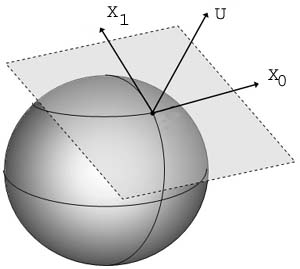
The normal to the surface at a point is given by
U = X0 x X1 / abs(X0 x X1)
The 2nd derivative is, by the chain rule,
a' '(s) = x0''*X0 + x0'*dX0/ds + x1''*X1 + x1'*dX1/ds
dX0/ds is evaluated along the curve, and we don't have an expression for it. We'll need a result from multi-variable calculus to analyze it further. Taylor's theorem for several variables (note: the one variable version is covered in CWT Vol. 3) can be used to show that
dXi/ds = ∂Xi/∂x0*x0' + ∂Xi/∂x1*x1'
Now the fun can begin: with the notation ∂Xi/∂xj = Xij, note that Xij is not necessarily in the tangent plane, so, we will separate it into its in plane and out of plane components, defining the functions
Grij , and Lij, so that
X00 = G000 X0 + G100 X1 + L00U
X01 = G001 X0 + G101 X1 + L01U
X10 = G010 X0 + G110 X1 + L10U
X11 = G011 X0 + G111 X1 + L11U
These are Gauss's equations. Note that Gi10 = Gi01 and L01 = L10. Now we can write
a'' = (x0'' + G000x0'2 + 2G001x0'x1' + G011x1'2)X0 +
(x1'' + G100x0'2 + 2G101x0'x1' + G111x1'2)X1 +
(L00x02 + 2L01x0x1 + L11x12)U
The Christoffel Symbols
The Grij symbols above are called Christoffel symbols of the second kind. We also have Christoffel symbols of the first kind defined by Gijk = Xij·Xk. The following 'three card monte' shows that the Christoffel symbols are functions of the metric coefficients; we will make use of this computing a solution to the field equations below: Differentiating
∂gik/∂xj = ∂(Xi·Xk)/∂xj = Xij·Xk + Xkj·Xi = Gijk + Gkji
Permutting indices yields
∂gkj/∂xi = Gkij + Gjik
and,
∂gji/∂xk = Gjki + Gikj
Subtracting the third equation from the sum of the first two gives
Gijk = (1/2)*(∂gik/∂xj + ∂gjk/∂xi - ∂gij/∂xk)
and by the lemma above
[Gijk] = [g]-1[Gijk]
The Equations of Weingarten
Since U · U = 1, the partial derivatives of U, denoted by Ui, are in the tangent plane and can be written, defining the functions Lij, as Ui = L0iX0 + L1iX1. These are the equations of Weingarten.
Since U · Xj = 0, differentiating both sides wrt xk gives
U · Xjk + Uk · Xj = 0, so that
Uk · Xj = - U · Xjk = -Ljk
And, from the lemma,
[-Lij] = [g] [Lij] so that [Lij] = [g]-1[-Lij]
The Riemann-Christofel Curvature Tensor
Hang in there, we've almost arrived. We will differentiate Gauss's equations with the goal of developing some equations for the second derivatives. Differentiating
Xij = G0ij X0 + G1ik X1 + LijU
wrt xk gives
Xijk = dG0ij/∂xkXij + G0ijX0k + dG1ij/∂xkX1 + G1ijX1k + LijkU + LijUk
Using Gauss's equations to write Xrkas a linear combination of X0 , X1 and U, and Weingarten's equations to write Uk as a linear combination of X0 and X1, and rearranging the terms gives
Xijk = (∂G0ij/∂xk + G0ijG00k + G1ijG01k - LijL0k)X0 + (dG1ij/∂xk + G0ijG00k + G1ijG11k - LijL1k)X1 + (.......)U
Exchanging j and k gives
Xikj = (∂G0ik/∂xj + G0ikG00j + G1ikG01j - LikL0j)X0 + (dG1ik/∂xj + G0ikG00j + G1ikG11j - LikL1j)X1 + (.......)U
Since Xijk = Xikj, subtracting the 1st equation from the 2nd gives
0 = ∂G0ik/∂xj - dG0ij/∂xk + G0ikG00j + G1ikG01j - G0ijG00k - G1ijG01k - LijL0k + LikL0j
and
0 = ∂G1ik/∂xj - dG1ij/∂xk + G0ikG10j + G1ikG11j - G0ijG10k - G1ijG11k - LijL1k + LikL1j
Defining Rhijk = ∂Ghik/∂xj - ∂Ghij/∂xk + G0ikGh0j + G1ikGh1j - G0ijGh0k - G1ijGh1k
we have
Rhijk = LikLhj - LijLhk
The Rhijk are the components of the Riemann curvature tensor. Note that the Riemann curvature tensor is defined in terms of the Christoffel symbols, which are functions of the metric coefficients. The Lij and Lij are functions of how the normal vector U changes, i.e., the curvature of the surface. Gauss defined the curvature of a 2-d surface geometrically, and showed that it equals det([L])/det([g]). The Riemann curvature tensor allows the curvature to be computed from values that can be calculated in the surface, the gij. It provides the building blocks for the left side of Einstein's field equations.
The Ricci Tensor and Einstein's Field Equations
It's time to get down to business. As is our wont, we will simplify things as much as possible by considering a 1-d world, giving 2-d spacetime. Einstein's field equations for empty space are
Rij = 0
where Rij = R0ij0 + R1ij1
The Rij are the components of the Ricci tensor.
Our goal now is to solve these equations for a world containing a single point mass M surrounded by a vacuum. The 16 components of the Riemann curvature tensor are:
R0000 = ∂G000/∂x0
- ∂G000/∂x0
+ G000
G000
+ G100
G010
- G000
G000
- G100
G010 (= 0)
R1000 = ∂G100/∂x0
- ∂G100/∂x0
+ G000
G100
+ G110
G010
- G000
G100
- G100
G110 (= 0)
R0100 = ∂G010/∂x0
- ∂G010/∂x0
+ G010
G000
+ G110
G010
- G010
G000
- G110
G010 (= 0)
R1100 = ∂G110/∂x0
- ∂G110/∂x0
+ G010
G100
+ G110
G110
- G010
G100
- G110
G110 (= 0)
R0010 = ∂G000/∂x1
- ∂G001/∂x0
+ G000
G001
+ G100
G011
- G001
G000
- G101
G010
R1010 = ∂G100/∂x1
- ∂G101/∂x0
+ G000
G101
+ G110
G011
- G001
G100
- G101
G110
R0110 = ∂G010/∂x1
- ∂G011/∂x0
+ G010
G001
+ G110
G011
- G011
G000
- G111
G010
R1110 = ∂G110/∂x1
- ∂G111/∂x0
+ G010
G101
+ G110
G111
- G011
G100
- G111
G110
R0001 = ∂G001/∂x0
- ∂G000/∂x1
+ G001
G000
+ G101
G010
- G000
G001
- G100
G011
R1001 = ∂G101/∂x0
- ∂G100/∂x1
+ G001
G100
+ G111
G010
- G000
G101
- G100
G111
R0101 = ∂G011/∂x0
- ∂G010/∂x1
+ G011
G000
+ G111
G010
- G010
G001
- G110
G011
R1101 = ∂G111/∂x0
- ∂G110/∂x1
+ G011
G100
+ G111
G110
- G010
G1001
- G110
G111
R0011 = ∂G001/∂x1
- ∂G001/∂x1
+ G001
G001
+ G101
G011
- G001
G001
- G101
G011 (= 0)
R1011 = ∂G101/∂x1
- ∂G101/∂x1
+ G001
G101
+ G111
G011
- G001
G101
- G101
G111 (= 0)
R0111 = ∂G011/∂x1
- ∂G011/∂x1
+ G011
G001
+ G111
G011
- G011
G001
- G111
G011 (= 0)
R1110 = ∂G111/∂x1
- ∂G111/∂x1
+ G011
G101
+ G111
G111
- G011
G101
- G111
G111 (= 0)
Eight of the Riemann curvature tensor components are identically 0. The components of the Ricci tensor are
R00 = R0000 + R1001 = R1001
R01 = R0010 + R1011 = R0010
R10 = R0100 + R1101 = R1101
R11 = R0110 + R1111 = R0110
Solving the Equations
A few weeks after Einstein published the general theory in 1915, he received a letter from Karl Schwarzchild , a German astrophysicist, who was fighting on the Russian front. The letter contained a solution to the field equations for a single point mass located in empty space. This solution is now known as the Schwarzchild solution. We can simplify it by considering a space of only 1 dimension, and the resulting spacetime with 2 dimensions.
We assume that the coordinates are orthogonal, so that g01 = g10 = 0; and we define functions m and n so that g00 = em and g11 = -en. The formula for the Christoffel symbols becomes
Gijk = 1/(2gii)(∂gji/∂xk + ∂gki/∂xj - ∂gkj/∂xi)
giving
G001 =
G010 = 1/(2g00)(∂g01/∂x0 + ∂g00/∂x1 - ∂g01/∂x0) = 1/(2g00)(∂g00/∂x1) = m'
G100 = 1/(2g11)(∂g10/∂x0 + ∂g01/∂x0 - ∂g00/∂x1) = 1/(2g11)( - ∂g00/∂x1) = - m'e2m - 2n
G111 = 1/(2g11)(∂g11/∂x1 + ∂g11/∂x1 - ∂g11/∂x1) = 1/(2g11)(∂g11/∂x1) = n'
G000 =
G011 =
G101 =
G110 = 0
The 1st field equation is
0 = R00 = R1001 = ∂G101/dt
- ∂G100/∂x
+ G001
G100
+ G101
G010
- G000
G101
- G100
G111
that is,
0 = 0 + d( - m'e2m - 2n)/∂x + m'm'e2m - 2n + 0*0 - 0*0 + n'm'e2m - 2n
0 = (- m'' + n'm' - m'2)e2m - 2n
and R01 and R10 are identically 0, and R11 is equivalent to the 1st.
The differential equation
- m'' + n'm' - m'2 = 0 is solved by inspection by m = (1/2)ln(a + bx), n = -(1/2)ln(a + bx)
so the solution is g00 = a + bx, g01 = g10 = 0 and g11 = -1/(a+bx)
Geodesics and the Curvature of Spacetime
 Let's compute the radius of curvature for Kareem's hook shot. In 1-d space, he'll have to shoot the ball straight up and then it will fall straight down.
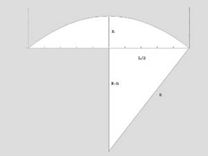
Suppose it is launched upward with a velocity of 10 m/sec, so it will travel upward for one second, reaching a height of 5m, and then descend for one second. Note that we will compute the arc of the ball's worldline in spacetime, not the 'frozen' arc of the ball in space only. The worldline arc is plotted to the right, but, not to scale. Note that the t axis units are seconds (time), and the x axis units are centimeters (distance). To use the same units on both axes, we need to convert to common 'geometric units' by convereting the time units to distance, and the conversion factor is c, the speed of light (3x1010 cm/sec). Thus, if drawn to scale, the horizontal axis would be 2*3x1010 units long. The arc should be beginning to look more straight now. We can compute the approximate radius of curvature: the arc is a parabola, but we will approximate it by a circle. We have
Let's compute the radius of curvature for Kareem's hook shot. In 1-d space, he'll have to shoot the ball straight up and then it will fall straight down.
Suppose it is launched upward with a velocity of 10 m/sec, so it will travel upward for one second, reaching a height of 5m, and then descend for one second. Note that we will compute the arc of the ball's worldline in spacetime, not the 'frozen' arc of the ball in space only. The worldline arc is plotted to the right, but, not to scale. Note that the t axis units are seconds (time), and the x axis units are centimeters (distance). To use the same units on both axes, we need to convert to common 'geometric units' by convereting the time units to distance, and the conversion factor is c, the speed of light (3x1010 cm/sec). Thus, if drawn to scale, the horizontal axis would be 2*3x1010 units long. The arc should be beginning to look more straight now. We can compute the approximate radius of curvature: the arc is a parabola, but we will approximate it by a circle. We have
(R - h)2 + (L/2)2 = R2 and R = (h2 + (L/2)2)/2h
setting L = 2*3x1010 and h = 500 gives a curvature of (1/R) = 7.5*10-18
The gravitational acceleration for an earth like mass is -980 cm/sec2 = -G = -10/c*c = -10-20
In flat spacetime, a straight line is a straight line, in curved spacetime, a straight line is a line whose curvature is solely due to the curvatue of spacetime, such a curve is called a geodesic. Recall the formula for the second derivative of a curve in a surface,
a'' = (x0'' + G000x0'2 + 2G001x0'x1' + G011x1'2)X0 +
(x1'' + G100x0'2 + 2G101x0'x1' + G111x1'2)X1 +
(L00x02 + 2L01x0x1 + L11x12)U
The curvature in the surface is represented by the in plane components of a''; thus a curve is a geodesic if and only if
x0'' = - (G000x0'2 + 2G001x0'x1' + G011x1'2)
and
x1'' = - (G100x0'2 + 2G101x0'x1' + G111x1'2)
We will substitute t for x0 and x for x1. The ' above represents differentiation wrt arc length, and, since ∂x << dt, we can omit the terms on the right side of the equations involving x', thus we have for a geodesic, with a = 1 and b = 2G
t'' = - G000t'2 = 0
x'' = - G100t'2 = -(-1/2g11)∂g00∂x = (1/2g11)(2G) = -G
From the first equation, t'' is 0 so that t is a constant multiple of arc length; the constant is very close to 1 since the arc length and change in t are nearly the same, thus approximately t' = 1. From the second equation, approximating g11 with -1, we have ∂x2/dt2 = -G, thus we have arrived at a DE for the trajectory of the ball, that is
∂x2/dt2 = -G
and this is similar to the Newtonian result.
Note that the downward acceleration of the ball does not depend on the ball's position, in contrast to gravity as we know it where the acceleration increases as the ball falls due to the increasing strength of gravity. The reason is the following: in 3-d, as the distance from a mass increases the gravitational force decreases in such a way that when integrated over a ball of radius r, the result is a constant. Thus, the force decreases proportional to 1/r2. In a 2-d world the gravitational force decreases proportional to 1/r. In a 1-d world it doesn't decrease.
References
Richard L. Faber, "Differential Geometry and Relativity Theory", Marcel Dekker, 1983