Differentiating Polynomials

Polynomials are engineers' favorite functions because they are easy to calculate. First we complete our study of the calculus of polynomials.

If p(t) = f(t)·g(t), then why doesn't p'(t) = f '(t)·g'(t)?

Here's why: think of f(t)·g(t) as the area of a rectangle with width f(t) and height g(t). Then, as t increases from t to to 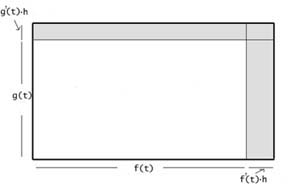t+h, the increase in f(t) is f'(t)*h, the increase in g(t) is g'(t)*h, and the increase in the size of the rectangle (shown shaded in the figure) is ~
f(t)·g'(t)·h + g(t)·f '(t)·h + f '(t)·g'(t)·hh,

The increase divided by h, that is, the rate of increase, is
f(t)·g'(t) + g(t)·f '(t) + f '(t)·g'(t)·h

which approaches f(t)·g'(t) + g(t)·f '(t) as h goes to zero.

Thus, p'(t) = f(t)·g'(t) + g(t)·f '(t).

This is the product rule for derivatives and can be used to easily determine the derivative for any power of t, and hence for any polynomial.

Polynomial Approximation and Taylor's Theorem

The linear approximation to a function matches the value of the function and the 1st derivative of the function. A linear function is a degree 1 polynomial. The n^th degree polynomial approximation to a function matches the value of the function and the 1^st n derivatives of the function. The n^th degree polynomial approximation to f(t) at t = 0 is given by
p(t) = f(0) + f'(0)*t + (1/2)*f''(0)*t² + (1/3*2)*f'''(0)*t³ + ... + (1/n!)*f⁽ⁿ⁾(0)*tⁿ

(Check that p(0) = f(0), p'(0) = f'(0), p''(0) = f''(0), etc.)

Taylor's theorem gives a bound on the error of the approximation as t moves away from 0. Polynomial approximation and Taylor's theorem are important because they provide a method for calculating the values of transcendental functions (functions other than polynomials) like the exponential and trigonometric functions, as we show below.

Quick proof of Taylor's theorem: the n^th degree polynomial approximation p(t) to a function f(t) at t = 0 is constructed so that p(0) = f(0), p⁽ⁱ⁾(0) = f⁽ⁱ⁾(0) for i <= n. Let e(t) = f(t) - p(t), then e⁽ⁱ⁾(0) = 0 for i <= n, and e⁽ⁿ⁺¹⁾(t) = f⁽ⁿ⁺¹⁾(t). Suppose f⁽ⁿ⁺¹⁾(t) < M for some interval 0 <= t <= h. Now, e⁽ⁿ⁾(0) = 0 and the rate of increase of e⁽ⁿ⁾(t) is < M, so e⁽ⁿ⁾(t) < M*t. And thus, e^(n-1)(0) = 0 and the rate of increase of e^(n-1)(t) is < M*t, so e^(n-1)(t) < M*t²/2. And thus, e^(n-2)(0) = 0 and the rate of increase of e^(n-2)(t) is < M*t²/2, so e^(n-2)(t) < (1/2)*M*t³/3. And so on, so that e(t) < (1/(n+1)!)*M*tⁿ⁺¹. Believe it or not the above is way simpler than anything you'll find in a textbook.

Here's the country version of this proof: if your old hound's maximum acceleration is M, and he runs for t seconds, than at most he has reached a velocity of M*t, n'est pas? So, he has travelled at most (M*t)*t. Had it been the hound's maximum 'jerk' (rate of change of acceleration) that was M, then, by the same argument, the hound's max acceleration at time t would be M*t, the hounds max velocity M*t*t, and the hound's max distance M*t*t*t. This is the basic principle underlying Taylor's theorem. (It only takes a little refinement to get the denominator (n+1)! ).

The Fundamental Theorem of Calculus

The Fundamental Theorem of Calculus (FTOC) is, succinctly,
= p(t2) - p(t1)
Thinking of p(t) as a position function, the right side of the equation is the distance traveled in the interval t1 to t2. If p(t) represents constant velocity motion, then the area corresponding to the integral is a rectangle, the height of the rectangle p'(t) = V, and the base of the rectangle is t2 - t1. Thus the area is V*(t2 - t1), and the FTOC is equivalent to the familiar formula velocity*time equals distance, V*(t2 - t1) = p(t2) - p(t1).

If p'(t) is a step function, then the area corresponding to an integral of p'(t) is a sum of 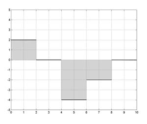rectangles, one for each subinterval, and the formula area = velocity * time = distance holds for each subinterval. Summing the areas of the rectangles gives the value of the integral.
An anti-derivative p(t) to the step function above is shown below. Summing the distances gives p(t1+h) - p(t1) + p(t1+2h) - p(t1+h) + p(t1+3h) - p(t1+2h) + ........ +p(t2) - p(t2-h) and the inner terms cancel ('telescope') so that the sum equals p(t2) - p(t1).

The integral of p' equals the sum of the areas for each subinterval, and that equals the sum of the distances for each subinterval, and that equals p(t2) - p(t1). Thus, the FTOC is true when p'(t) is a step function

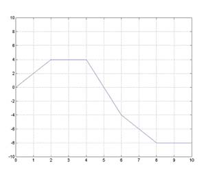
Let p'(t) be any function with anti-derivative p(t), then a step function can be constructed so that it is arbitrarily close to p'(t). An example is shown to the left.
The antiderivative of the step function is then arbitrarily close to p. The antiderivative of the step function above is graphed along with p to the left. Since the FTOC is true for the step function, it easily follows that the FTOC is true for p'(t).

Roots and Radicals

It's easy to define the meaning of fractional exponents. For example, y^1/2 is the square root of y, that is the number that when multiplied by itself equals y. Similarly, the cube root of y, y^1/3, is the number that when multiplied by itself two times equals y. However, calculating the value of a fractional exponent is usually not so easy. 5^1/2=?. Here is a surprise: while we can't directly calculate most of the values for a function like p(t) = t^1/2, we can differentiate the function. Note that if q(t) = t², then q(p(t)) = t. Differentiate both sides, using the chain rule to differentiate the left side. Now with a hop, skip and jump we show that [t^1/2]' = 1/2t^-1/2. Similarly for t^1/n for any positive integer n. Another use of the chain rule gives [t^m/n]' = m/n t^{m/n -1} for any positive integers m and n. If we can't directly calculate values of fractional exponent functions (or exponentials or trig functions), how does our calculator do it? Read on.

Exponentials and Logarithms

If the exponent is the variable, we have an exponential function, e.g. p(t) = 10^t is the base 10 exponential function. It's easy to show from the definition of a derivative that p'(t) = p'(0)*p(t), and we deduce the existence of a number e such that the base e exponential function exp(t) = e^t has exp'(0) = 1 and hence exp'(t) = exp'(0) * exp(t) = 1 * exp(t). So, before you can say Jack Spratt, we differentiate exp(t) to get exp(t) = exp'(t) = exp''(t) = exp'''(t).... etc., and we can write the polynomial approximation to exp(t) at t = 0 as
f(t) = 1 + t + (1/2)*t² + (1/3*2)*t³ + ... + (1/n!)*tⁿ.

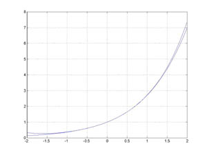
exp(t) is shown with its 4th order polynomial approximation in the figure.

The natural log function is the inverse of exp, that is ln(exp(t)) = t. We use the chain rule to show that the derivative of ln(t) is 1/t. We know the derivatives of all orders for 1/t, so we can construct polynomial approximations to ln.

The values of exp and ln are calculated by using polynomial approximation. Ln and exp can then be used to calculate the values of fractional exponents.

exp(t) is one of nature's favorite function because it 'looks like' its derivative, and that makes it a prime candidate to be a solution to the homogeneous differential equations that play a part in the analyses of most physical systems. We analyze first order systems occuring in mechanics and electrical circuit theory.

Trigonometric Functions

The basics of plane trigonometry are covered in five lessons, with the goal of defining the sine and cosine functions, and deriving the trigonometric identity needed to differentiate them (sin(A + B) = sin(A)*cos(B) + cos(A)*sin(B)).

Using this identity the derivative of sin(t) at t = a is the limit of (sin(A+h) - sin(A))/h = (sin(A)*cos(h) + cos(A)*sin(h) - sin(A)) / h as h approaches 0. As h approaches 0 cos(h) approaches 1 and sin(h) approaches h, so, the limit is (sin(A)*1+ cos(A)*h - sin(A)) / h = cos(A). Similarly, cos'(t) = -sin(t). From the definitions, sin(0) = 0 and cos(0) = 1, so the (2n+1)th order polynomial approximation to sin(t) is
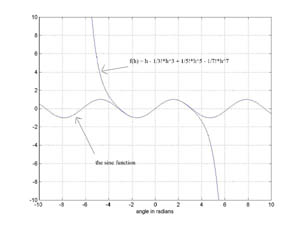
f(t) = 0 + t - (1/3*2)*t³ + (1/5*4*3*2)*t⁵ + ... + (-1)ⁿ(1/(2n+1!)*t²ⁿ⁺¹.

sin(t) is shown with its 7th order polynomial approximation in the figure.

Values of trig functions are calculated using polynomial approximation.

We have sin'(t) = cos(t) and sin''(t) = -sin(t), so that the second derivative of sin(t) is a multiple of sin(t), and sin(t) is also a candidate solution for a homogeneous differential equation. We defer examples to the next chapter.

Second Order Systems

Linear second order systems are used to model a wide variety of physical phenomena, and are basic building blocks of engineering analysis. The differential equation for a linear second order system can be written p''(t) + u*p'(t) + K*p(t) = f(t), with all the terms containing a derivative of p on the left side and the 'forcing function' f on the right. If the forcing function is replaced by 0 we have the homogeneous form of the equation; this equation characterizes the unforced motion of the system. It is 'homogeneous' because all the terms contain p or a derivative of p. Exponential and trig functions provide the solution, hence, they are nature's favorites, and they figure in almost every engineering analysis.

Analyzing the spring mass assembly shown in the figure, we start with F=MA and let M=1 for simplicity. 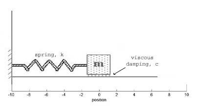The forces acting on the block are gravity and the force of the table pushing up on the block, which cancel, and the forces due to friction (-u*p'(t)) and the spring (-K*p(t)) where u is the coefficient of friction and K is the spring constant. So, the differential equation for the system is p''(t) + u*p'(t) + K*p(t) = 0

In the case where the spring is strong, i.e., K² - (u/2)² > 0, the solution to the DE, 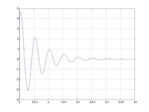and the motion of the block, is damped oscillation and is the product of an exponential and a sine wave, with p(t) = A*exp(-l*t)sin(wt + o). The solution can be rewritten, using our favorite trigonometric identity from the previous chapter, as p(t) = B*exp(-l*t)*(B*sin(wt) + C*cos(wt). Using this form it is easy to solve for the constants B and C to meet the given initial conditions. An example of damped oscillation is shown in the figure.

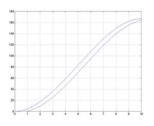
In the case where the spring isn't so strong, i.e., K² - (u/2)² < 0, the system doesn't oscillate and has a solution that is a sum of exponentials of the 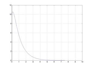form p(t) = A*exp((a+b)*t) + B*exp((a-b)*t). A representative solution is shown in the figure.

To analyze the circuit in the diagram we use Kirchoff's voltage law, which states that the sum of 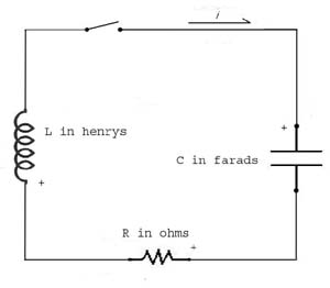the voltages around a closed loop is 0. The equation characterizing the inductor is v_L(t) = L*i'(t) where v_L is the voltage across the inuction, L is the inductance of the inductor, and i is the current in the loop. The equation characterizing the resistor is v_R(t) = R*i(t) where v_R is the voltage across the resistor and R is the resistance of the resistor. The equation characterizing the capacitor v_C(t) = 1/C&int:i(t) where v_C is the voltage across the capacitor C is the capacitance of the capacitor. Kirchoff's voltage law is v_L + v_R + v_C = 0, that is
L*i'(t) + R*i(t) + 1/C&int:i(t) = 0
differentiating both sides yields
i''(t) + (R/L)*i'(t) + (1/LC)*i(t) = 0
Wait a minute, this differential equation is mathematically identical to the one for the spring-mass assembly, the only things having changed are the names of the function, variables and constants. So, the solutions are the same.