Calculus Without Tears

The Wave Equation

Introduction

In the CWT texts we analyze motion problems using Newton's Second Law, and electrical circuits using the differential equations that characterize electrical components along with the relevant circuit laws. In this page we will see how the techniques we have studied can be applied to analyze wave motion.

The basic physics/engineering paradigm is: start by analyzing the system and writing the differential equations that characterize it, then solve the differential equations, so that's what we'll do. We'll see that the wave equation can be derived from physical principles we've already studied plus the ideal gas law.

In the traditional curriculum we would then proceed to solve the differential equation analytically. However, we don't want to get bogged down with difficult to solve DEs, but we do want to see how the wave equation works. So, we will solve it numerically with a FREEMAT program, as is shown below. Duck soup!

Calculus with Multiple Variables

For simplicities sake, CWT only deals with functions of one variable. We can't represent a wave whose amplitude changes with position and time with a function of just one variable, as we need variables to represent both position and time. Waves occur in 3-dimensional space, and it takes 3 numbers to represent a position in 3-dimensional space, so we can represent an acoustic wave with a function p(x,y,z,t) where x,y, and z are spatial coordinates and t is time, and p(x,y,z,t) is the displacement in the equilibrium pressure at the point x, y, z at time t.

By considering one dimensional waves we will be able to limit ourselves to functions of two variables in what follows. Below we will use a two variable function p(x,t) where x is a location variable and t is time. When we have functions of more than one variable, derivatives are called 'partial derivatives'. For example the function v below is a function of two variables, x and t,
    v(x,t) = 3*x² + x*t²

By considering x to be a constant the function becomes a polynomial with one variable, t, and we can differentiate it wrt t, and the result is called the partial derivative of v wrt t and is denoted by , that is is the name of the derivative, and
    (x,t) = x*2*t,
(remember, x is constant so 3*x² is a constant and has derivative 0, and the derivative of x*t² wrt t is x*2*t).
Similarly, by considering t to be a constant we can differentiate the function wrt x to get the partial derivative of v wrt x, given by
    (x,t) = 6*x + t²

We can take 2nd order partial derivatives
= = = x*2
= = = 2*t
= = = 6
= = = 2*t
Note that
    =
We will use this important property of partial derivatives on this page and on the general relativity page.

Also, note that is just the name of a function, (we could have named the function "Fred" if we were inclined to defy convention), that is obtained by first taking the partial derivative of v wrt t and then taking the partial derivative of that function wrt x. We have introduced a fancy notation, but the concept of derivative hasn't changed at all, it is identical to what is covered in CWT Vol. 2. The s and s have no intrinisic meaning, they are just used to write the conventional names for partial derivative functions.

The Wave Equation

The wave equation characterizes wave motion in gas, liquids, and solids, as well as electromagnetic waves. We'll examine the acoustic case, this equation describes how sound waves propagate in air.

We will show one derivation of the wave equation in this section, and another in the section on Maxwell's equations. There is also a different and very concise derivation at Wave equation - Wikipedia, the free encyclopedia, this derivation uses springs and masses.

A Derivation of the Acoustic Wave Equation

The Ideal Gas Law

We will need the ideal gas law from chemistry which is P · V = m · R · T, where
    P = pressure
    V = volume
    m = mass
    R = the universal gas constant = 287 J·kg^-1·K^-1
    T = temperature in degrees Kelvin

The ideal gas law says that (at a fixed temperature) the pressure of the gas in a fixed volume is directly proportional to the mass of the gas, that is, as the mass increases the pressure increases, and as the mass decreases the pressure decreases. As you pump air into the tire the pressure increases, as you let air out it decreases. No big surprise.

A One Dimensional Physical Model

We'll keep the number of spatial dimensions to 1 by assuming that we have a very small straight hollow tube filled with air, and that the air moves only in the direction of the tube. We will study the motion and the pressure of air in the tube.

The constant P will represent the equilibrium pressure, that is, atmospheric pressure. The function p(x,t) will represent the displacement from the equilibrium pressure due to an acoustic wave at location x at time t.

The function v(x,t) will represent the velocity of the air in the tube at location x at time t. When no wave is present v(x,t) = 0 for all x.

The Acceleration of Air in the Tube

The image below represents a thin hollow tube filled with air. The x variable measures position along the length of the tube. 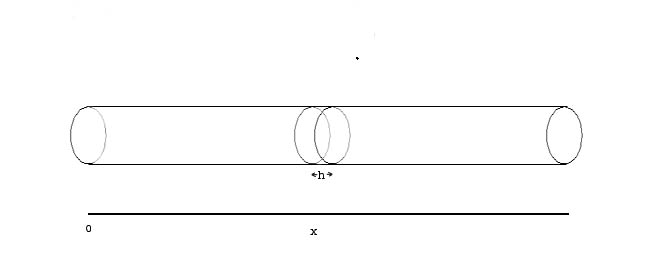The cross sectional area of the tube is A and is very small.

The volume of the air in the tube segment between x and x+h is V_s = A*h.

Consider the forces acting on the air in this segment time t. From the left, the force equals p(x,t) ·A, and from the right the force is p(x+h,t) ·A (note that the forces due to P cancel). So the total force is [p(x,t) - p(x+h,t)] ·A.

From Newton's 2nd Law of Motion F = m ·Acceleration, so, the acceleration of the air between x and x+h is given by F / m, that is,
    = [p(x,t) - p(x+h,t)]·A / m_s

From the ideal gas law we have m_s = P·V_s / R·T, so
    = [p(x,t) - p(x+h,t)] ·A · R · T / P · V_s

Note that A / V_s equals 1/h, so, as h -> 0 the above equation becomes
    = - · R·T / P

That is, a spatial pressure 'differential' causes the air in the tube to accelerate.

The Time Derivative of Pressure

Air flows into the left side of the segment at x to x+h at the rate v(x,t)·A and flows out the right side at the rate v(x+h,t)·A. Thus the total rate of the the air flowing into the segment is
   [v(x,t) - v(x+h,t)] ·A

This will produce a change in the pressure in the segment. First we convert the volume rate to a mass rate. From the ideal gas law the density of the air is m / V = P / R·T , so the mass rate into the segment is
   [v(x,t) - v(x+h,t)] ·A·P / R·T

Now we will convert the mass rate into a pressure rate. From the ideal gas law, the ratio of pressure to mass in the segment is R·T / V_s, so we have
    = [v(x,t) - v(x+h,t)] ·A·P / R·T · [R·T / V_s] = [v(x,t) - v(x+h,t)] ·A·P / V_s

Note that A / V_s is 1/h. As h -> 0, the above equation becomes
    = - · P

That is, a spatial velocity 'differential' causes pressure to increase or decrease.

The Second Time Derivative of Pressure

Taking the second partial derivative of pressure wrt time gives
    = - · P

Taking the partial derivative of acceleration wrt x gives
    = - · R·T / P

Noting that = and substituting gives the wave equation
    = · R·T

OK, Let's See What This Wave Equation Can Do

With the wave equation in hand, we can study the propagation of sound in air. We will stay with our 1-dimensional model of a thin hollow tube. Since the differential equation for p is a second order equation, we'll need to specify initial values of p and . In the examples below we'll start with p and equal to 0 for all values of x and t = 0.

We will generate a disturbance the left end of the tube (x = 0) by specifying p(0, t) as time progresses.

We will use the method we used in CWT Vol. 2 Ch. 2 to compute the solution to the wave equation. We'll divide the length of the tube into short segments of length h, and divide time into short interval of duration dt. Since the differential equation for p is second order we'll first calculate an estimate of using the wave equation, and use it to project forward, then we'll use that value to project p forward, using our favorite formula distance = velocity * time, or more generally, change = rate of change * time.

All but three lines of this FREEMAT progam are programming details, but, we can't avoid them. We'll need arrays to store the values of p(0, h, 2h, 3h, .......) and dpdt(0, h, 2h, 3h, .......), so we have
   p = zeros(1,1000);
   dpdt = zeros(1,1000);
And, it will be easier if we have an array for the temporary storage of results, so
   pL= zeros(1,1000);

We initialize our constants
   R = 287;
   T = 300;        % room temperature Kelvin
   h = 1;             % 1 meter
   dt=0.00001;   % a small time step
   n=25000;        % we'll run the sim for 1/4 seconds

And away we go .... the outer i loop advances time, the inner j loop advances position
   for i = 1:n;       % t=i*dt
       for j=1,100            % x=(j-1)*h
           if (j == 1)

Here comes the disturbance signal at the left end of the tube
               p(1) = sin(2*pi*i*dt*10);        % a 10 hertz sine wave
           else

We can estimate the first derivative of pressure wrt location (x) at jh plus a smidge by (p(j+1) - p(j)) /h, and at jh minus a smidge by (p(j) - p(j-1)) /h.
Then we use these estimates to estimate the 2nd derivative of pressure wrt x, and the wave equation to estimate the 2nd derivative of pressure wrt time; this is all shown in the next line.
               d2pdt2 = R*T*[(pL(j+1) - pL(j)) /h + (pL(j) - pL(j-1)) / h] / h;    % the wave equation
               dpdtnew = dpdt(j) + d2pdt2*dt;                 % change in dpdt = rate of change of dptdt * time
               p(j) = pL(j) + (dpdtnew + dpdt(j))*dt / 2;       % change in p = rate of change of p * time
               dpdt(j) = dpdtnew;
           end
        end
        pL = p;      % bookkeeping
   end

The plot of p below represents the air pressure displacement from equilibrium in the tube after running the simulation for 0.25 seconds.

   plot(p(1:100))