When Newton discovered gravity, he then understood the force pulling the apple to earth; and that the same force holds the moon in its orbit. But, he didn’t have any way of determining the trajectory of the apple or the moon. He would need a new type of mathematics, the mathematics of motion.

Calculus Is Easier than You Think

Calculus is the mathematics of motion. In this volume we restrict ourselves to the simplest type of motion, constant velocity motion, and we see that calculus for constant velocity motion is simple indeed.

Calculus in a nutshell is the formula distance equals velocity times time, or distance = velocity * time. Surprisingly, you won't discover this in your high school or college calculus courses. Let's look in more detail:

Differential calculus is the calculation of derivatives, or, in plain English, velocities. Well, velocity = distance / time does it (for constant velocity motion).

Integral calculus is the calculation of the area under a velocity curve for a given interval. A velocity curve (for constant velocity motion) is a horizontal line, and the area under the curve is given by the formula for the area of a rectangle, that is, height * length. The height of the velocity curve is the velocity, the length of the interval is the time, and hence, the value of the integral is velocity * time.

The Fundamental Theorem of Calculus states that the integral of a velocity curve for a time interval is the distance traveled in the interval. Well, we've seen that the value of the integral is velocity * time, so the Fundamental Theorem of Calculus is velocity * time = distance (for constant velocity motion).

Differential equations are, in plain English, velocity equations. If we have an equation for, that is, know, the velocity for constant velocity motion, and we know the starting position of the motion, it is easy to use the formula distance = velocity * time to compute the position of the motion, that is, to solve the differential equation.

Is all this a parlor trick? No, the calculus of constant velocity motion really is the foundation for all calculus, and Calculus Without Tears is the only calculus method that presents the fundamentals in this easy to understand way, in CWT Volume 1, Constant Velocity Motion. We go beyond constant velocity motion in Volumes 2 and 3.

Representing Motion Mathematically - Functions

The concept of a mathematics of motion is a tremendous leap from the arithmetic that preceded calculus. First, how is motion represented mathematically? The usual concepts from arithmetic, counting and measuring, are insufficient. You can’t ‘count’ motion, or use a ruler and ‘measure’ it.

Motion is a complex process that involves changing time and changing position. What we need is a way to represent the relationship between time and position for the motion.

Mathematics uses functions to represent change. Suppose a runner starts on the 0 yard line, and runs at a constant velocity of 5 yards per second. Then, the runner's position at the instant at time t is given by evaluating the expression 5 * t and this expression embodies the relationship between time and position for the runner's motion.

The notation p(t) == 5 * t associates the name p with the function calculated by the expression 5 * t (and thereby 'defines' the function p). It is usually more convenient to refer to a function by its name rather than writing out the expression itself.

Suppose the runner starts (at time t = 0) on the 10 yard line and runs with a velocity of 3 yards per second. Then, the function representing the runner’s motion is p(t) == 3 * t + 10.

Suppose the runner starts on the 30 yard line but doesn’t run at all. Then the function representing the runner's position is p(t) == 30.

The functions above are pretty simple. Of course, not all functions are so simple. It is possible to write a function that fills up an entire line with obscure symbols representing difficult operations. But, in essence, simple and complex position functions representing motion do the same thing: they compute a position for each value of time. In CWT Vol. 1 we stick with simple motion and simple functions.

If the above is new to you, take a break after finishing this section. Using functions to represent motion is probably the highest hurdle in this volume. Perhaps, after the break, read this section for the second time. When it seems familiar, proceed on to the next section.

Representing Motion Graphically – Graphs

Operations in calculus are performed on functions, and it is sometimes helpful to have a graphical representation of the function in order to better understand the effect of the operation. Also, graphs play an essential part in integral calculus (discussed below). 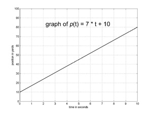From a graph representing a runner’s motion, we can determine the runner’s position at each instant in time.Thus, the graph contains the same information as the function. The graph to the left represents the motion of a runner who starts on the 10 yard line and runs with a velocity of 7 yards per second for 10 seconds. The function representing the runner’s motion is p(t) == 7 * t + 10. The graph is a straight line. The runner’s starting position equals p(0) and can be read from the graph at the intersection of the graph and the vertical axis (the vertical line above t=0). The slope of the graph is calculated as the change in position divided by the change in time, and equals the runner’s velocity.

Calculating Velocity – Derivatives

The crux of calculus is calculating velocity. That is, given a function that represents motion by calculating a position for each instant of time, we want to find the function that represents the velocity of the motion by calculating a velocity for each instant. A function that represents velocity is called a derivative. Calculating derivatives is what calculus is all about.

If a function is simple, it is easy to calculate its derivative (velocity). Let’s start with the simplest case: if the runner is standing still, his velocity is 0. So, if p(t) == C for some constant, then the runner’s velocity, which we'll usually denote by p’(t), is always 0, that is, p’(t) == 0. Viola’, we have differentiated (found the derivative for) our first function. Using the name p’ for the function that is the derivative of p is purely a matter of convention; and there is no special significance to the ' symbol, it's just part of the name.

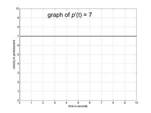
If the runner is running at a constant velocity V, then the runner’s velocity is V at each instant. So, if p(t) == V * t, then p’(t) == V. Changing the runner’s starting position does not change the runner’s velocity, so, if p(t) == V * t + P0, then p’(t) still equals V. Now we’ve differentiated a whole class of functions, the linear functions (functions with straight line graphs).

It’s been a little too easy thus far. We’ll hit the first speed bump in calculating derivatives in Volume 2 (calculating the derivative for p(t) == t*t) but it will only slow us down for a minute.

Calculating Areas – Integrals

Calculus can also be used to calculate the area of irregular shapes; a special symbol is used to indicate the area under a graph, it is called the integral symbol and it looks like an elongated script S. The area under the graph of a function f for the interval t1 to t2 is indicated by

  Note that there is nothing magical about this symbol; it is just used to indicate the area under a curve, and, it doesn't give any clues as to how this area is to be calculated.

Now, we've stacked the deck in Vol. 1.... consider the area under the velocity curve for constant velocity motion. The graph is a horizontal line, so, the area is a rectangle and we can use the standard formula 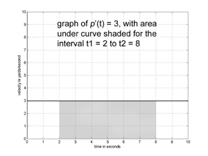for the area of a rectangle to evaluate the integral.

A graph of the velocity function p’(t) == 3 is shown to the left, with the area beneath the graph for the interval t1 to t2 shaded gray.

This area is a rectangle so we can calculate its area by using the formula for area of a rectangle, that is, height times width. The height of the rectangle is 3, and its width is t2 – t1, so the area is 3 * (t2 – t1). So, we've shown that

= 3 * (8 - 2) = 18

If p is a position function and p’ is its velocity function, then there is an important connection between p and the area under the graph of p’. This connection is so important it is called the Fundamental Theorem of Calculus, which is

= p(t2) – p(t1)

For constant velocity motion, we just showed that the left side is evaluated by area = velocity * time; for any motion the right side is end position - start position, that is, distance traveled, so the Fundamental Theorem of Calculus, applied to constant velocity motion, is the familiar formula velocity * time = distance.

We have shown that the Fundamental Theorem of Calculus is true for constant velocity motion. The demonstration that it is true for any motion is an easy extension of the method used above, but there is a little speed bump, so it will be deferred to Volume 3. The important thing to grasp now is the basic idea, that is, the area under a velocity curve equals distance traveled, it is true for all types of motion.

Differential Equations

Calculus without differential equations is like a car without wheels, you can't get very far. A differential equation is an equation that contains a derivative, and a derivative is, in plain English, a velocity, so a differential equation is, in plain English, a velocity equation.

Suppose p is a position function, but, we don't know the equation defining it. It is unknown! Nonetheless, by convention its velocity is named p', and we can write an equation for it
p'(t) = 5, for example.
This is a differential equation. We have an equation for the velocity function, but we don't know the position function. Note that the derivative name is bold in the above equation, we write it this way to remind ourselves that p is an unknown function.

To solve the differential equation means to come up with a definition of p that satisfies the differential equation, that is, that makes it true. For this example, that means coming up with a definition of p(t) so that p'(t) = 5

Now, it's on you. Can you solve this differential equation? Take a minute. Can you come up with a definition of p(t) so that p'(t) = 5 ?

Suppose I define p with the equation p(t) == 7*t + 20, then, does p'(t) = 5, that is, does it satisfy the differential equation above? Can you change it so that it does?

A solution is p(t) == 5*t + 20. Well, how about p(t) == 5*t + 30? Yes, that's a solution too. Changing the position function by changing its starting position does not affect its velocity function, so many position functions will satisfy the differential equation.

The First Differential Equation

When an apple falls to earth the force of gravity pulls it. Exactly how does this force affect the apple's trajectory? Newton answered this question with his Second Law of Motion, which states that F(orce) = M(ass) * A(acceleration). For a falling apple, we know the force, that is gravity, and we know the mass of the apple, so, using the equation A = F / M, we can compute the apple’s acceleration.

Suppose the apple's position is given by the function p(t). At this point, we don’t know the equation defining p. We write p in bold type to remind us that we don’t know how to compute it at this point. Even thought we don't know the equation defining p, we know, by convention, the name of the derivative of p, and so the name of the apple's velocity function is p’(t).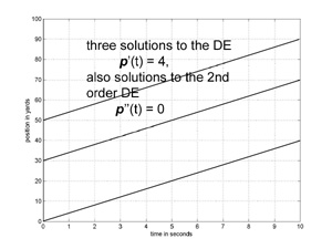

The rate of change of velocity, that is the derivative of velocity, is acceleration. By convention the name of the derivative of p'(t) is p''(t), so p’’(t) is the name of the apple's acceleration function. From Newton’s Second Law of Motion, we know that p’’(t) = F / M. This is an example of a differential equation (DE). A differential equation is an equation that contains the derivative (a second derivative in the example above) of an unknown function (p is unknown in the sense that all we have specified is its name, we don’t know the equation that defines it).

We’ll solve the above DE in Volume 2, for now, consider an easier case: suppose no forces are acting on the apple, then p’’(t) = F / M = 0 / M = 0. Can you solve this differential equation? That is, can you come up with an equation defining p(t) so that p’’(t) = 0? Well, how about a position function for constant velocity motion? Consider, if p(t) == V * t + P0, then p’(t) = V, that is the runner's velocity is constant, and so the runner's acceleration is 0, that is p’’(t) = 0. So any constant velocity motion p has zero acceleration and solves the DE p’’(t) = 0.